
We can perform many methods to visualize and analyze multivarate data. In the tutorial you can find scripts and a short description to 3 of the most commonly used ones:
- Cluster analysis
- Multi dimensional scaling (MDS)
- PCR/RDA
In this post, we will go through Cluster analysis.
For each method, there are some variations. You can (and should) test several analysis, transformations and settings and compare them. Right now, this is a preliminary version. It uses some of your own dataset (one for benthos, one for algae; you find it on the student server under “data analysis”). It shoudl cover most of what you need for your projects.
I have also included some plot settings for customized plots of the analysis. Hopefully, this will be extended with a proper tutorial soon.
The analysis are rund with using the following libraries:
[code language=”r”]
# libraries ####
library("vegan") #package written for vegetation analysis
library("MASS") # ‘MASS’ to access function isoMDS()
library(stats) # e.g for hclust() function
[/code]
Before starting, remember to set your working directory, and import your files. For those analysis you need observations in rows, variables in columns and unique rownames. The example data in this script can be found on the student server adn the script for import as well.
We start with clustering. Cluster analysis is used to find groupings in a set of observations (clusters) that share similar characteristics. For example comparing a series of samples whith multiple measured variables. Exactely what we often want to do in community analysis when comparing different communities either from different areas or at different point in time.
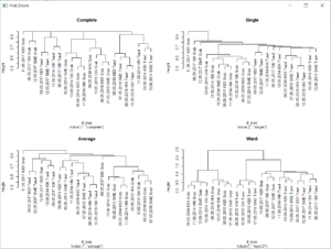
A cluster analysis produces a cluster-diagram, called dendrogram, that looks like a tree. There are many clustering methods. Here, one of the more commonly methods, agglomerative hirachical clustering, is presented.
Before we can run hclust(), on of the available functions for cluster analysis, we need to prepare a distance matrix, which calculates similarities between sampling units based on the species composition
[code language=”r”]
d_bray <- vegdist(B_taxa.4thrt,method="bray") #Bray Curtis similarity, common in community analysis; the data used is a fourth root transformed data set with benthic taxa
[/code]
Now, we can run the cluster anlysis, using hclust() in library(stats). it is made to performe hierarchical cluster analysis on a set of dissimilarities and for methods to analyzing the resulting trees. Through the function we can use different clustering methods.
[code language=”r”]
#compare different clustering methods
treeBC_g <- hclust(d_bray) #complete linkage standard
treeBC_gs <- hclust(d_bray,method="single") #single linkage
treeBC_gw <- hclust(d_bray,method="ward.D") #Ward clustering
treeBC_ga <- hclust(d_bray,method="average") #average linkage
#and plot the different trees for comparison
par(mfrow=c(2,2)) #set plotting area so we can compare all 4 plots
plot(treeBC_g, main="Complete")
plot(treeBC_gs,main="Single")
plot(treeBC_ga, main="Average")
plot(treeBC_gw,main="Ward")
par(mfrow=c(1,1))
[/code]
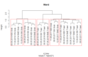
After inspecting the clusters, we can overlay the cluster with boxes for the foudn groups. The number of groups has to be given in the function.
[code language=”r”]
plot(treeBC_gw,main="Ward")
rect.hclust(treeBC_gw,5)
grp <-cutree(treeBC_gw,5)
[/code]
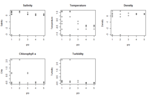
After we found groups, we can plot them (or alternatively test them) against environmental variables.
[code language=”r”]
par(mfrow=c(2,3))
plot(Salinity~grp,data=B_envir.st, main="Salinity")
plot(Temperature~grp,data=B_envir.st, main="Temperature")
plot(Density~grp,data=B_envir.st, main="Density")
plot(Chla~grp,data=B_envir.st, main="Chlorophyll a")
plot(Layer_m~grp,data=B_envir.st, main="Depth")
plot(Turbidity~grp,data=B_envir.st, main="Turbidity")
par(mfrow=c(1,1))
[/code]
We can also overlay those groups on an ordination plot, like an MDS.