
We can perform many methods to visualize and analyze multivarate data. In the tutorial you can find scripts and a short description to 3 of the most commonly used ones:
- Cluster analysis
- Multi dimensional scaling (MDS)
- PCR/RDA
In this post, we will go through Multidiemnsional Scaling – or short MDS.
For each method, there are some variations. You can (and should) test several analysis, transformations and settings and compare them. Right now, this is a preliminary version. It uses some of your own dataset (one for benthos, one for algae; you find it on the student server under “data analysis”). It shoudl cover most of what you need for your projects.
I have also included some plot settings for customized plots of the analysis. Hopefully, this will be extended with a proper tutorial soon.
The analysis are rund with using the following libraries:
[code language=”r”]
# libraries ####
library("vegan") #package written for vegetation analysis
library("MASS") # ‘MASS’ to access function isoMDS()
library(stats) # e.g for hclust() function
[/code]
Before starting, remember to set your working directory, and import your files. For those analysis you need observations in rows, variables in columns and unique rownames. The example data in this script can be found on the student server adn the script for import as well.
Multi Dimensional Scaling (MDS)
Multidimensional scaling – or MDS – i a method to graphically represent relationships between objects (like plots or samples) in multidimensional space. To reduce this multidimensional space, a dissimilarity (distance) measure is first calculated for each pairwise comparison of samples. Those are plotted onto 2 or 3 dimensional space, in such a way, that distances between points on the plot approximates their multivariate dissimilarity as closely as possible. If we talk about samples and species composition this means: points – representing 1 sample each – which are located closely together on the plot have more similar species composition then samples located far from each other on the plot. MDS, like cluster analysis or PCA, is one of the methods commonly used to compare communities based on their species composition.
With MDS, we can create an ordination plot from any measure of similarity or dissimilarity among samples. There are many different ways of calculating dissimilarity among samples. The simplest, but not very well suited for community data, is Euclidean distance (i.e., the straight-line distance between two points in multivariate space). For species composition, the most commonly used distance measure is the Bray-Curtis dissimilarity/similarity index. Bray-Curtis is better at handling the large proportion of zeroes (e.g., species absences) commonly found in ecological data sets then many other measures (shared absence is NOT considered as similar).
There are also several classes of MDS – nonmetric MDS and classical or metric MDS.
Non-metric MDS (nMDS) is a non-parametric rank-based method. It is comparatively robust to non-linear relationships between the calculated dissimilarity measure and the projected distance between objects. Often, it gives a better – more unbiased – visual representation than other methods, like metric MDS or PCA, which is described later. To get an overview over your data, I would start with a nonmetrica MDS first. Below, there are scripts for both non-metric and metric MDS, but with focus on the non-metric MDS.
Before starting with an MDS, there are some additional data preparations steps, that might be nessecarry, depending on your data.
[code language=”r”]
#remove columns and rows with only 0
B_taxa <- B_taxa[which(rowSums(B_taxa)>0),] #subsetting, rowSums() calculates the sum of each row, a logical argument removes rows with only 0
#remember to remove corresponding rows in environmental data if nesscessary
rownames(B_taxa) #check rownames files to compare
rownames(B_envir.st)
names(B_taxa) #check columnnames files to compare
names(B_envir.st)
#check that all parameters are numeric, and change if needed (e.g. integer to numeric)
str(B_envir.st)
# to make plotting easier and to be able to have good labeles, it might be worth assigning shorter column names
[/code]
### nonmetric MDS ####
## With isoMDS in MASS ####
Since MDS projects distances between samples, we start with preparing a distance matrix by calcualting distances/dissimilarities between rows (samples). Here, we use the Bray Curtis dissimilarity and the function vegdist() in library(vegan)
[code language=”r”]
d_bray <- vegdist(B_taxa, method="bray")
[/code]
Now, we can performe our MDS, using isoMDS() in library(MASS). Usually, I recommend to rather use metaMDS in library(vegan), which is explained a bit further down.
[code language=”r”]
fit <- isoMDS(d_bray,k=2) # k is the number of dim
fit # view results
[/code]
..and plot the results. (see further below for the different plotting settings).
[code language=”r”]
plot(fit$points[,1], fit$points[,2], xlab="Coordinate 1", ylab="Coordinate 2", main="Nonmetric MDS", type="n")
points(fit$points,pch=19,cex=1,col=as.numeric(B_envir$Method))# plots sample points; stratification depth color-coded; this can be interchanged with other nominal variable e.g. gear or station or year; for details ?points
text(fit$points[,1], fit$points[,2], labels = row.names(B_taxa), cex=.7)
[/code]

If you remember from earlier: the closer the points representing each sample are together on the plot, the more similar in species composition they are.
## With metaMDS in vegan ####
The metaMDS function in vegan uses several random starts to find stable solution and standardizes the scaling. It might not work on small datasets. Using the metaMDS function, the distance-matrix does not need to be claculated beforehand. The function calculates the distance matrix and the community-dataframe works as data-input. You can choose between several distance measures.
One can also call decostand() within meta(). decostand() performs a data transformation. It includes e.g. a hellinger transforamtion, an alternative to the pre-performed 4th root transformation (see script for import of data and data-preparation). Below, metaMDS is performed with different choices
[code language=”r”]
mMDS1 <-metaMDS(decostand(A_taxa,"hellinger"),distance = "euclidean",k=3,engine = c("isoMDS"),trymax = 100,autotransform =F)
mMDS <- metaMDS(A_taxa^(1/2^(3-1)),distance = "bray",k=2,engine = c("monoMDS"),trymax = 100,autotransform =F)
[/code]
The standard function for plotting various ordinations in vegan is ordiplot(). The standard plot might look at bit messy, but it can be customized.
[code language=”r”]
ordiplot(mMDS, type ="t")
[/code]
There are other ways of plotting an MDS, which in my opinion make it easier if you want to customize the plot. I mostly use the base-R functions for plotting and customization (but you could also use ggplot).
[code language=”r”]
#remember: par () sets up the plotting area, here you define rows and columns to plot in; e.g. mfrow=c(2,2) is 2 plots in 2 rows (=4 plots)
par(mfrow=c(1,1),mar=c(3, 3, 3, 10),pch=20,xpd=TRUE) # create a grip for several plots and leae space fo a margin on one side
palette(c("blue","red","green3","orange","black"))#reates a custome color palett which is used in the plot
#now we create the plot
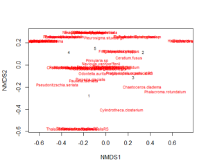
plot(mMDS,display = c("sites","species"),type="n",shrink=T) #create empty plot area first; more freedom for how you plot elements
points(mMDS,pch=as.numeric(Alga$Species),cex=1,col=as.numeric(Alga$Strat.strength))# adds layer with samples; stations symbol-coded, stratification depth color-coded; this can be interchanged with other nominal
text(mMDS, "species",col="blue", cex=0.7)# adds species, species are placed in the same space as samples. So species in the right pper corner are more common in samples in the right corner of the plot.
[/code]
We can also add a legend to the plot using legend() and text().
[code language=”r”]
#The location of the legend in relation to MDS axes: the first 2 numbers in the brackets
#find the right place for legends adn text by adjusting the x and y values
#see ?legend for settings
legend(0.45,0.3,c("1","2","3","4","5"),lty=c(1,1,1,1),col=c("black","red","green","orange","blue"),cex=0.8)
legend(0.45,0.1,c("A","B"),col=c("black","black"),pch=c(2,1))
text(0.3,0.25,"fit: R2=???",cex=0.8)
text(0.3,0.2,"Stress=???",cex=0.8)
[/code]
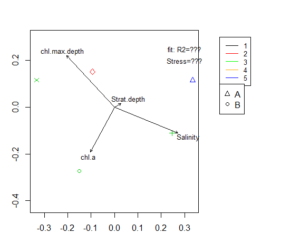
Fitting of environmental variables is done by the envfit() function. It is the most commonly used method of interpretation for MDS results. Environmental vectors are fitted onto the ordination. Those arrows points to the direction of most rapid change in the the
environmental variable and the length of the arrows is proportional to the correlation between ordination and environmental variable.
[code language=”r”]
#### check fit and significance of environmental variables ####
ef <- envfit(mMDS, A_envir.st, permutations=9999) #creates table with stats; if few observations, you will get a warning, but can still have results
ef2 <- envfit(mMDS ~ Salinity + chl.a, A_envir.st) #it is also possible to only fit a few variables
ef #you can find p and r2 values in the table that is returned
ef2
#and plot the fitted variables on the MDS diagram
plot(envfit(mMDS, A_envir.st),col="black",cex=0.8)
[/code]
We have several other options to include environmental data in our MDS plot. Below, there are codes for some of them to further customize your MDS plot and add additional information. Since some of those option include statistical procedures, they need a sufficiently large or good dataset to work on.vegan provides several other plotting possibilities for including environmental data.
[code language=”r”]
# Color coding according to
plot(mMDS, display = "sites",type="n")
points(mMDS,pch=as.numeric(Alga$Species),cex=1)
#overlay for continuous variables with ordisurf() (works only with larger datasets)
chl <- with(A_envir.st, ordisurf(mMDS, chl.a, add = TRUE, col = "green4",lty=4)) #creates extra layer; nested function – more advanced coding
chl
with(A_envir.st, ordisurf(mMDS, Salinity, add = TRUE,col="darkgrey"))
#MDS plots with color coding for continous variable with colour ramp ####
#create colour ramp – for example if you have many samples along a gradient, this can be useful
colourful&lt;- colorRampPalette(c("red4","red","orange","Yellow","green"))
points(mMDS,pch=as.numeric(Alga$Species),cex=1,col=colourful(length(Alga$chl.a)))# plots samples; stations symbol-coded, chla color-coded
text(mMDS, "species",col="blue", cex=0.7)#this might be useful in some cases
plot(envfit(mMDS, A_envir.st),col="black",cex=0.8) #plot fitted environmental variables on top; length of arrow according to correlation with composition
[/code]
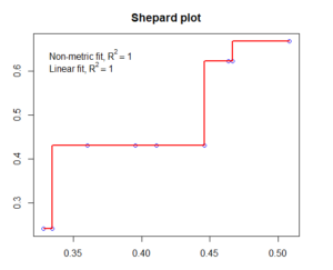
You can check how good the MDS-representation in several ways. One is a stressplot.
[code language=”r”]
stressplot(mMDS,main="Shepard plot")
#there are several other methods to verify your MDS, but this is outside the scope of our course. See links on the bottom of the post.
[/code]
## #Classical metric MDS ####
The function wcmdscale() is a weighted analysis, and results are identical to PCA-results with rda function in vegan.
We start with preparing a distance matrix by calcualting distances/dissimilarities between rows in vegdist() again. In the script below, several distance matrices are produced from the same data, using different Euclidian distance and Bray Curtis dissimilarity.
[code language=”r”]
#for example with algae
d_bray <- vegdist(A_taxa, method="bray") #vegan function, can calculate several similaritys/distances
d_eucl <- dist(A_taxa) # stats function, standard euclidean distances; usually not for species data unless with prior transformation in CA/PCR
#for example with benthos
d_bray <- vegdist(B_taxa, method="bray")
d_eucl2 <- dist(B_taxa)
[/code]
Now we can preform an MDS. For illustration we do this with all 4 examples
[code language=”r”]
fit <- cmdscale(d_eucl,eig=TRUE, k=2) # k is the number of dimensions we want to represent our data on; see also ?cmdscale
fit # call results
fit1 <- cmdscale(d_bray,eig=TRUE, k=2)
fit1
fit2 <- cmdscale(d_bray2,eig=TRUE, k=2)
fit2
fit3 <- cmdscale(d_eucl2,eig=TRUE, k=2)
fit3
[/code]
I want to plot the solutions for the different MDS together, so it is easier to compare. So we need to set up our plotting environment first. This id done using par().
[code language=”r”]
par(mfrow=c(1,2), mar=c(3, 3, 3, 3))
# mfrow=c() defines the number of plots in rows and columns
#mar=c() defines the margins around each plot
[/code]
Now we can plot our results with several MDS in a grid.
[code language=”r”]
# for algal example
plot(fit$points[,1], fit$points[,2], xlab="Coordinate 1", ylab="Coordinate 2", main="Metric MDS", type="n") #this line prepares the plot areas
points(fit$points,pch=c(19,19,19,19,19),cex=1,col=as.numeric(Alga$Strat.strength))# adds a layer with points each representing one sample
# the stratification depth is color-coded using col=as.numeric(Alga$Strat.strength)); can be substituted by other nominal variable e.g. gear or station or year
text(fit$points[,1], fit$points[,2], labels = row.names(A_taxa), cex=.7) #might be obsolete, adds a lable for each sample in the respective spot over the point
plot(fit1$points[,1], fit1$points[,2], xlab="Coordinate 1", ylab="Coordinate 2", main="Metric MDS", type="n")
points(fit1$points,pch=c(19,19,19,19,19),cex=1,col=as.numeric(Alga$Strat.strength))
text(fit1$points[,1], fit1$points[,2], labels = row.names(A_taxa), cex=.7)
#for benthos example
plot(fit3$points[,1], fit3$points[,2], xlab="Coordinate 1", ylab="Coordinate 2", main="Metric MDS", type="n")
points(fit3$points,pch=as.numeric(B_envir$Station),cex=1,col=as.numeric(B_envir$Method))# stratification depth color-coded; can be substituted by other nominal variable e.g. gear or station or year
plot(fit2$points[,1], fit2$points[,2], xlab="Coordinate 1", ylab="Coordinate 2", main="Metric MDS", type="n")
points(fit2$points,pch=as.numeric(B_envir$Station),cex=1,col=as.numeric(B_envir$Method))
par(mfrow=c(1,1), mar=c(3, 3, 3, 3)) #resetting plot-environment to 1 plot per figure
[/code]
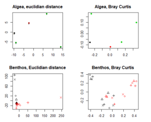 The resulting MDS differ. As you can see for the benthos, Bray Curtis dissimmilarity performes by far better and gives us more inforamtion.
The color-coding in the upper two MDS indicate different station.
n the lower two MDS, stations are indicated by different symbols, and gear type (grab samples and trawl samples) by different colors.
For more information and a longer tutorial on functions included in vegan, have a look here .
A good tutorial on the net to have a look at could also be this one.