9. Add a trendline to a data series

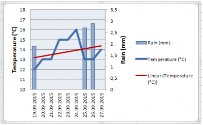
MS Excel offers an option to draw a trendline on top of your data series. This can be quite helpful to show a trend when the data is a bit to scattered to draw conclusions or when you want to simplify the “look” of your chart. To do so, click on your chart, go to the Layout tab of the Chart Tools and click on the icon Trendline. A dialog box shows up and asks you to choose a data series between those in use in the current chart. Here, choose the temperature series and click OK. A line pops up in the plot area. This line is an object which is fully configurable. Right click on it and choose Format Trendline to access various options. Among these options is the possibility to define which type of calculation MS Excel uses to define the trendline. Choose between Exponential, Linear, Logarithmic, and others, add a name, set the intercept if necessary and choose to visualize the equation and the R-squared value on the chart, then click OK.