
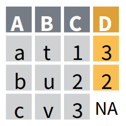
There is a family of four functions that allows for joining variables from two tables X and Y while matching values to the rows they correspond to. In other words, the functions check whether there are common rows and columns, before putting the data together. Depending of which of these functions you plan to use, you will be able to restrict the output table to only the observations that were found in X, only the observations that are common to both X and Y, only the observations that were found in Y, or retain all observations. This is called mutate joining, and the four functions are:
left_join(): join data while matching values from Y to X, keeping only the observations found in X,right_join(): join data while matching values from X to Y, keeping only the observations found in Y,inner_join(): join data, keeping only the observations which are common to both tables,full_join(): join data, keeping all the observations.
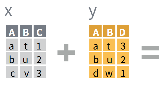
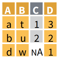
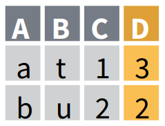
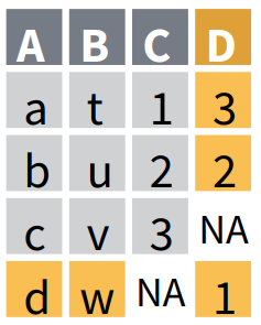
The icons found in Rstudio’s cheat sheet Data Transformation with dplyr : : CHEAT SHEET are of great visual help when trying to figure out the output of these “join” functions. We will keep them here as reference. These icons show what happens to 2 input tables X and Y (represented below) when handled by the 4 functions.
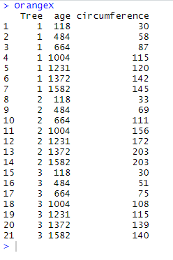
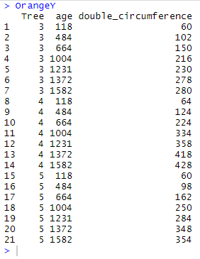
We will practically illustrate the use and purpose of the functions using OrangeX and OrangeY which are modified fragments of the data frame Orange. These fragments are generated using the following codes:
OrangeX <- Orange %>%
  filter(Tree == "1" | Tree == "2" | Tree == "3")
OrangeY <- Orange %>%
  filter(Tree == "3" | Tree == "4" | Tree == "5") %>%
  mutate(double_circumference = circumference*2)  %>%
  select(Tree, age, double_circumference)
and they look like this:
NB: as you may see here above, OrangeX and OrangeY have two variables in common: Tree and age; in addition, there are 7 common rows where Tree = 3.
Joining data while matching values from Y to X, keeping only the observations found in X with left_join()
left_join() returns a table with all the observations from the table X, and keeps all the variables found in X and Y. It keeps observations from Y only if they are found in X. The observations in X with no match in Y will have NA values in the new columns. If there are multiple matches between X and Y, all combinations of the matches are returned.
Let’s see that with OrangeX and OrangeY:
left_join(OrangeX, OrangeY)
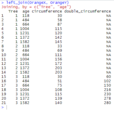
Here left_join() has restricted the output table to the 21 observations that are found in OrangeX, and has added the column double_circumference found in OrangeY. left_join has also found that there are 7 observations that are common to OrangeX and OrangeY, where Tree equals 3 and for which values in age match too. Therefore, it displays these 7 common observations with values for both circumference and double_circumference. Note that the other 14 observations have now the value NA in double_circumference since none of them was found in OrangeY.
Joining data while matching values from X to Y, keeping only the observations found in Y with right_join()
right_join() returns a table with all the observations from the table Y, and keeps all the variables found in X and Y. It keeps observations from X only if they are found in Y. The observations in Y with no match in X will have NA values in the new columns. If there are multiple matches between X and Y, all combinations of the matches are returned.
Let’s see that with OrangeX and OrangeY:
right_join(OrangeX, OrangeY)
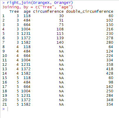
Here right_join() has restricted the output table to the 21 observations that are found in OrangeY, and has added the column circumference found in OrangeX. right_join() has also found that there are 7 observations that are common to OrangeX and OrangeY, where Tree equals 3 and for which values in age match too. Therefore, it displays these 7 common observations with values for both circumference and double_circumference. Note that the other 14 observations have now the value NA in circumference since none of them was found in OrangeX.
Joining data while keeping only the observations which are common to both tables with inner_join()
inner_join() returns a table with only the observations found BOTH in X and Y, and keeps all the variables found in X and Y. If there are multiple matches between X and Y, all combinations of the matches are returned.
Let’s see that with OrangeX and OrangeY:
inner_join(OrangeX, OrangeY)
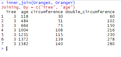
Here inner_join() has restricted the output table to the 7 observations that are found BOTH in OrangeX and OrangeY, and has kept all the variables found in OrangeX and OrangeY. It now displays these 7 common observations with values for both circumference and double_circumference.
Joining data while keeping all the observations with full_join()
full_join() returns a table with all observations and all variables from both X and Y, regardless of potential matches. Where there are not matching values, NA replaces the one missing.
Let’s see that with OrangeX and OrangeY:
full_join(OrangeX, OrangeY)
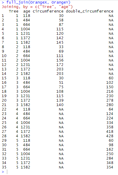
Here full_join() has opened the output table to all 21 observations that are found in OrangeX and all 21 observations found in OrangeY. It has detected 7 common observations where Tree equals 3 and for which values in age match too, and has thus merged them. full_join() has kept all the variables found in OrangeX and OrangeY. It now displays these 35 observations with values for both circumference and double_circumference, and with NA whenever a value is missing from one of the tables.