
Entire data frames may be put together either beside each other (thus increasing the number of variables) or below each other (thus increasing the number of cases) into a single, large table. Here we focus on combining data frames below each other.
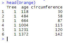
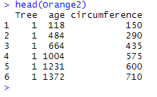
One of the functions that can do such an operation is bind_rows(). To illustrate how bind_rows() works, we will use the data frames Orange and Orange2 as examples. Orange2 is a data frame similar to Orange , with the difference that the values of the variable circumference have been multiplied by 5 using the following line of code:
Orange2 <- Orange %>% mutate_at(vars(circumference), list(~.*5))
We thus have the following two data frames Orange and Orange2:
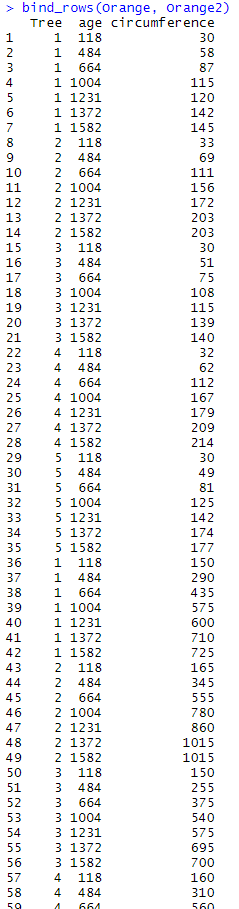
Note that the data frames have three identical variables: Tree, age, and circumference. We can combine the two data frames with the following code which gives :
bind_rows(Orange, Orange2)
which gives us a long table with 70 (2*35) rows, the first 35 rows being those from Orange and the last 35 rows being from Orange2:
The example above is rather simple since the variables in the data frames are the same. What if things were different?
Here is what happens when the data frames have (at least) one variable which is not common to both. Let’s use Orange3 which is similar to Orange, with the difference that the variable circumference has been renamed to circumferenceNEW using the following code:
Orange3 <- Orange %>% rename(circumferenceNEW = circumference)
head(Orange3)

And now we put them together:
bind_rows(Orange, Orange3)
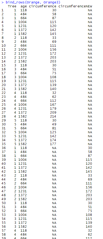
We end up with a 70 row-long table made of one more column than the original data frames, and that contains both circumference and circumferenceNEW. On top of that, the value NA has been placed whenever the observations did not have a value for the new variable.