dplyr has a handful of functions that allow for cleaning a data set by selecting a specific subset of observations. Here are the functions we will look at here:
filter(): extract rows that meet logical criteriaslice(): extract rows by positiontop_n: extract the rows containing the n highest/lowest values for a given variabletop_frac: extract a fraction of a data set where rows contain the highest/lowest values for a variablesample_n: extract n randomly-selected rowssample_frac: extract a fraction of randomly-selected rowsdistinct(): keep only unique rows (remove duplicates)
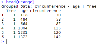
Let’s use the data frame Orange as an example. The top of the data frame looks like this:
head(Orange)
Extracting rows by criteria with filter()
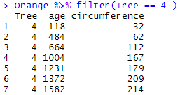
filter() allows you to retrieve from a data frame the rows (observations) which match logical criteria. Logical criteria are operations for which the result is TRUE or FALSE and which contain logical operators such as >, <, >=, >=, ==, !=, etc. For instance, to retrieve the observations that concern tree #4, we may write:
Orange %>% filter(Tree == 4 )
which results in:
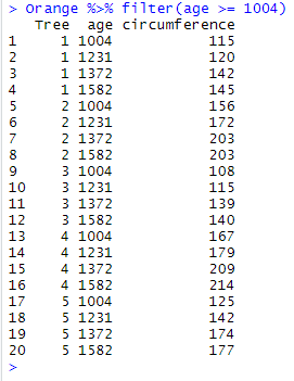
And to retrieve the observations that were performed since age 1004:
Orange %>% filter(age >= 1004)
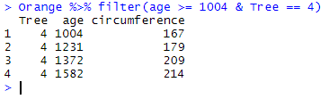
We may even combine logical criteria:
Orange %>% filter(age >= 1004 & Tree == 4)
Extracting rows by position with slice()
slice() allows you to retrieve from a data frame the rows (observations) which have a given position in this data frame.
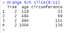
Here is how to retrieve the rows 8, 9, 10 and 11, regardless of their content:
Orange %>% slice(8:11)
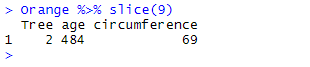
If slice() is only provided with a single value, it will pick up the corresponding rows in the data frame:
Orange %>% slice(9)
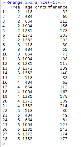
If slice() is provided with negative values, it will pick up the data frame but discard the corresponding rows:
Orange %>% slice(-1:-7)
Extracting a given number of rows containing the top/bottom values for a variable with top_n()
top_n() allows for retrieving the top or bottom n values in a data frame according to a given variable. If top_n() is only given a positive value n but no variable, it picks up the top n observations while considering the last variable in the data frame (and will indicated it in red):
Orange %>% top_n(10)
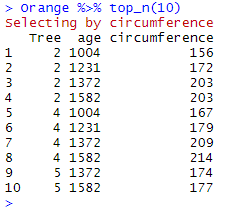
As expected, the console returns the 10 observations for which circumference (the last variable) is highest, and indicates “Selecting by circumference”.
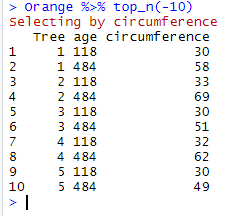
When top_n() is given a negative value n, it retrieves the bottom n values:
Orange %>% top_n(-10)
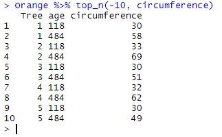
When top_n() is provided with a variable, it will extract the observations for which the n values are highest/lowest in that variable:
Orange %>% top_n(-10, circumference)
Note that top_n() may provide you with more than n rows than expected. If there are ties (i.e. several rows with equal values for the given variable), the function will give you all the observations matching the criteria. In the following example, we expect only 3 rows to be extracted by top_n():
Orange %>% top_n(3, age)
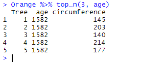
However the result tables comes with 5 observations for all of which age equals 1582, the highest value in the variable.
Extracting a fraction of a data set containing the top/bottom values for a variable with top_frac()
top_frac() works in a similar way to top_n(). It sorts the data frame by a given variable, and retrieves the rows with the top or bottom values. This time, unlike top_n() which retrieves a given number of rows, top_frac() retrieves a given percentage/fraction of the number of rows. In the following example, we ask for the top 20% of the rows sorted by the variable circumference:
Orange %>% top_frac(.2, circumference)
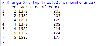
As expected we get 7 out 35 observations .
Again, if no variable is mentioned in top_frac(), the last variable is considered. If a negative value is given, the bottom rows will be selected. And if there are ties, all the observations with equal values are provided:
Orange %>% top_frac(-.2, age)
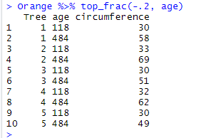
Here for instance, we got the 10 bottom rows when we only expected 7.
Extracting a given number of randomly selected rows with sample_n()
sample_n extracts a number n of rows which have been randomly picked from the data frame. Here is an example:
Orange %>% sample_n(5)
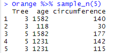
Since the selection is random, using twice the same code provides you with two different samples:
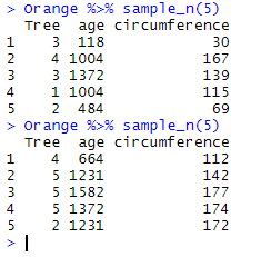
When randomly retrieving a large number of observations from a data frame, you may be given twice the same observation. sample_n() avoids this by using by default the argument replace = FALSE (i.e. you do not need to write the argument to make sure that all the picked observations are different). However, if, for some reason, you want to accept duplicates in your sample, you must add (replace = TRUE).
Extracting a given fraction of randomly selected rows with sample_frac()
sample_frac extracts a given fraction/percentage n of rows which have been randomly picked from the data frame. Here is an example:
Orange %>% sample_frac(.5)
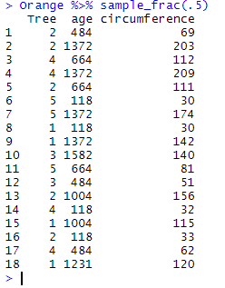
Again, since the selection is random, there is very little chance that using twice the same code will provide you with two identical samples.
When randomly retrieving a large fraction of a data frame, you may be given twice the same observation. sample_frac() avoids this by using by default the argument replace = FALSE (i.e. you do not need to write the argument to make sure that all the picked observations are different). However, if, for some reason, you want to accept duplicates in your sample, you must add (replace = TRUE).
Removing all duplicate rows with distinct()
distinct() is a function that checks the data frame for duplicate values for a (combination of) given variable(s) and thus returns only unique observations. In the following example, we will check Orange and retrieve only unique observation based on the variable circumference:
Orange %>% distinct(circumference)
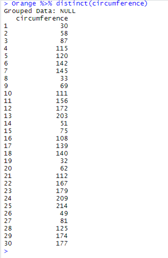
Out of the 35 original observations, distinct() has retrieved 30 rows, and thus discarded 5 rows where non-unique values were found in circumference. Note that the present table only shows the value in the column circumference, not the whole row. To keep the whole row and thus display all the corresponding variables, add the argument .keep_all = TRUE to your code:
Orange %>% distinct(circumference, .keep_all = TRUE)
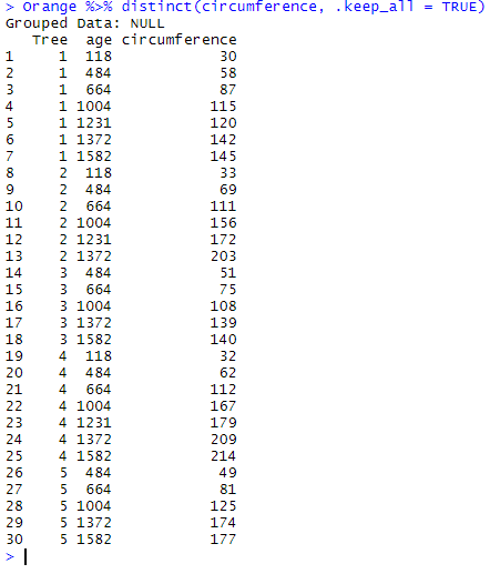
Both Tree and age now appear next to circumference in the output table.
Doing the same for Tree instead of circumference reduces even more the output:
Orange %>% distinct(Tree, .keep_all = TRUE)
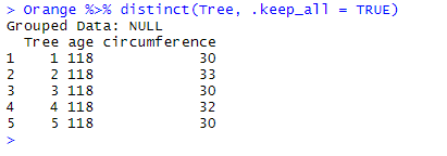
Only 5 observations have been kept by distinct(), and you can see that these were not randomly selected, but were the first rows from the top (based on age). You may thus be careful when using distinct() to “clean” your data frame as you may discard rows with potentially interesting content based on the fact that they had duplicate values in another column…
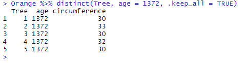
You may combine variables and logical operators to “force” distinct() to select another set of duplicate values when necessary. Here, we reuse the previous code, but add age = 1372 to keep only the duplicates for which age equals 1372, instead of those containing 118:
Orange %>% distinct(Tree, age = 1372, .keep_all = TRUE)