
If you wish to check that your dataset has been entered properly in Excel, you may use a couple of tools like Sort & Filter and Conditional Formatting.
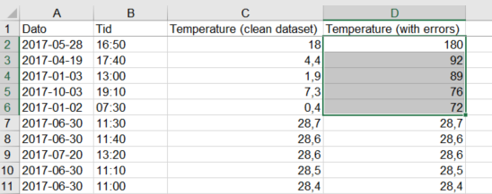
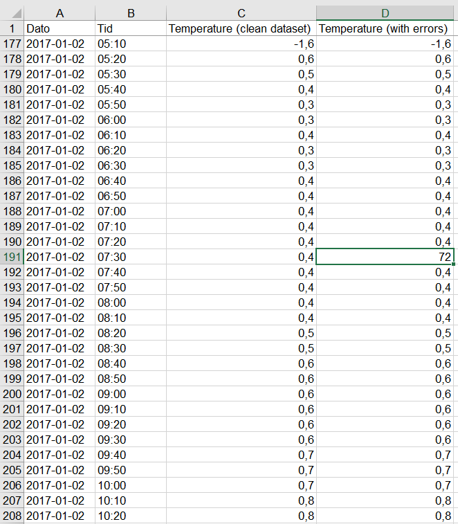 Here is an example where local temperatures have been retrieved from a weather station at Fløyen, in Bergen for the period 1/1/2017-31/12/2017 and placed in an Excel sheet. Since temperatures are retrieved from the station every 10 minutes, there are over 52000 values in total! It is virtually impossible to “manually” check that each and every data point in the table is correct or make sense. We thus need to find a way to spot the mistake more rapidly. Note: the column C contains the data that was retrieved; the column D contains the same data, but 5 aberrant data points (temperature between 70 and 200 degrees Celsius, see highlighted cell) have been inserted for the purpose of this example.
Using Sort & Filter
Aberrant data points such as extreme values or outliers (values that come either higher or lower than a certain range of values) may be spotted using a sorting function or tool. The goal is to reveal them by sorting the data in an ascending or descending order. Check here how to use Sort & Filter
 Select the columns A, B, C and D and click on
 Custom sort... in Sort & Filter. If your table contains headers, then tick off the My data has headers option. The name of your variables now appears in the sort by field. Select the variable Temperatures (with errors), then select values and largest to smallest, and click OK. Your selection has now been rearranged accordingly and shows the highest values on top, thus revealing extremely high values which are unlikely to match temperatures in Bergen. You may do the same with smallest to largest to reveal the lower values.
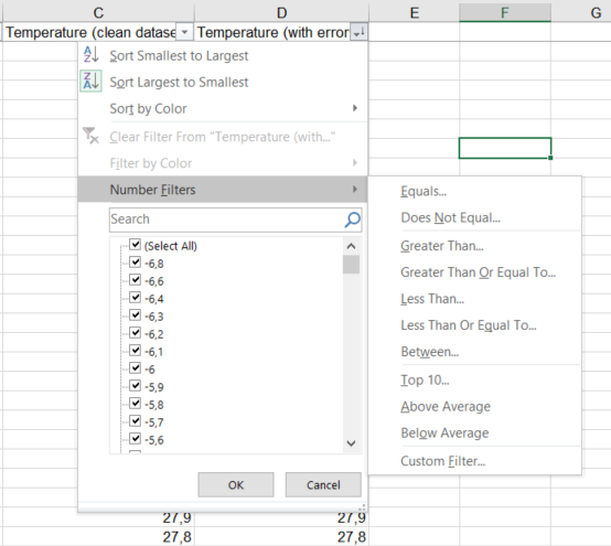 Similarly, you may use the
 Filter function. Select the columns A, B, C and D and click on Filter in Sort & Filter. Arrowheads appear immediately to the right in the cells of the header. By clicking on the arrowhead to the right of Temperatures (with errors), you may choose to sort the data in a similar way as for Custom sort... , or you can use Number Filters to refine/limit your display to top/bottom values for example, or to data greater or lower than a given value.
Using Conditional Formatting
Aberrant data points or cells containing data points may be given a different format (for example a different cell color) via the Conditional Formatting tool. Check here how to use this tool.
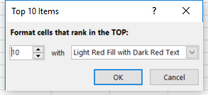
In our example, select the column of interest (column D: Temperatures (with errors)) and go to Conditional Formatting. Choose then which cells or values you would like to highlight (Top 10 items (see picture) or Top 10%, Bottom 10 items or Bottom 10 %, or anything else that makes sense for your analysis) and give these values/cells a specific color.
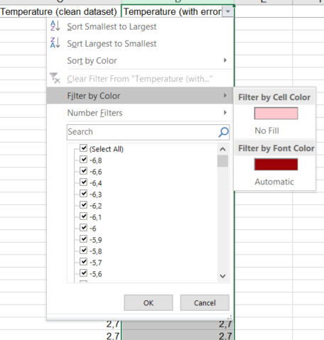 Then, use
 Filter as described above on column D and choose Filter by color. Click on the light red box under Filter by Cell Color. All the values that were marked by the Conditional Formatting tool in the previous step are now isolated. You may now check whether the data is aberrant or not.
Searching for empty cells or specific symbols
 Aberrant data is not only aberrant values; it may also be absence of value in a cell. Depending of where/how the data has been collected, absence of data is marked with N/A or NA or any other non-numerical character. But sometimes the cell is just empty.
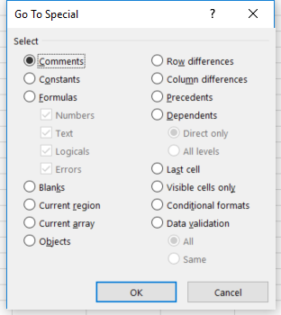
To spot empty cells, select the table/column of interest, use the Go To Special tool under Find & Select in the Home ribbon. Select then the Blanks option and OK. All empty cells are now highlighted.
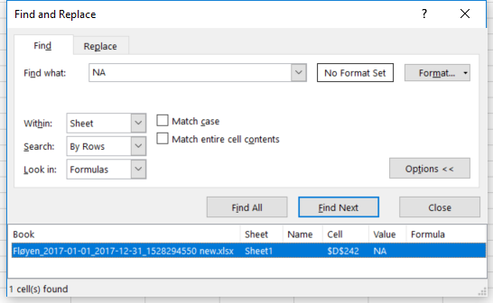 To find and highlight specific strings of characters (such as N/A or NA), press
 CTRL + F or go to Find & Select and then choose Find.... Next to Find what, type what you are searching for (such as NA) and click Find All. A table is now added to the dialog box that shows all occurrences and their address in the worksheet.