
The CTD data we are using comes in different formats. The .cnv files can be converted to text files by opening the .cnv files in notepad (this option comes up if you choose to use the standard Windows service) and then save them as text files.

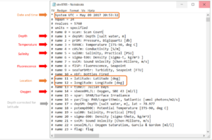
CTD files obtained from Helmer Hanssen cruises have running numbers – to see which station the CTD corresponds to see student reports as well as the station log from the bridge (date and time will let you know which fjord/station it is).
A lot of information about the CTD-profile is given in the header of the file wen you open it. For example the date and time and in which column you can find the data you are after:
There are several ways to prepare your CTD data. A good summary has been prepared for a course given in Bergen, which will be helpfull for you and can be found here.
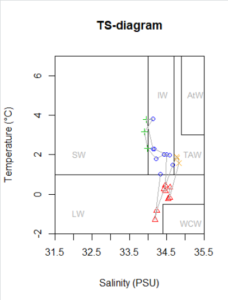
It is very useful to plot your salinity and temperature data into a TS-diagram.
The Temperature-Salinity diagram has salinity and temperatures on the x- and y- axis and the seperate measurements are plottet into this diagram. I here also included boxes for the different water masses watermasses according to Nielsen et al. 2008, so it is easy to find out what influence you have.
The script is a bit long and might seem daunting, but you can run it easily if you have the salinity and temperature values included in your main datafile as columns.
[code language=”r”]
setwd("C:/Users/x/OneDrive/AB202 vår 2019/R")
#### import data and preps ####
Mero<-read.table("C:/Users/x/OneDrive/AB202 vår 2019/R/Meroplankton.txt", header=TRUE, sep="\t", dec=",")
Mero$Julian_Day<-as.numeric(Mero$Julian_Day)
Mero$Date<-as.Date(Mero$Date, tz="UTM", format="%d.%m.%Y")
MeroW<-Mero[Mero$Layer=="whole",]
names(MeroW)
####TS-diagram (with water types indicated, according to Nielsen et al) ####
#with colorcoding for watermasses ####
#set figur area
palette(c("blue","red","green3","orange","black"))
#plot upper CTD measurements
plot(MeroW$"Salinity", MeroW$"Temperature",cex=1,col=as.numeric(MeroW$Season2),pch=as.numeric(MeroW$Season2), xlim=c(31.5, 35.5), ylim=c(-2, 7), xlab="Salinity (PSU)", ylab="Temperature (°C)", axes=F, main="TS-diagram")
polygon(c(34.7,34.7,35.5,35.5),c(1,7,7,1),col="white")#TAW
text(34.8,2, "TAW", cex=0.8, pos=4, col="darkgray")
polygon(c(34.9,34.9,35.5,35.5),c(3,7,7,3),col="white")#AtW
text(34.9,5, "AtW", cex=0.8, pos=4, col="darkgray")
polygon(c(31.5,31.5,34.0,34.0),c(1,7,7,1),col="white")#SW
text(31.8,2, "SW", cex=0.8, pos=4, col="darkgray")
polygon(c(34.0,34.0,34.7,34.7),c(1,7,7,1),col="white")#IW
text(34.1,5, "IW", cex=0.8, pos=4, col="darkgray")
polygon(c(31.5,31.5,35.5,35.5),c(1,-2,-2,1),col="white")#LW
text(31.8,-1, "LW", cex=0.8, pos=4, col="darkgray")
polygon(c(34.4,34.4,35.5,35.5),c(-0.5,-2,-2,-0.5),col="white")#WCW
text(34.7,-1.5, "WCW", cex=0.8, pos=4, col="darkgray")
points(MeroW$"Salinity", MeroW$"Temperature",pch=as.numeric(MeroW$Watermass),cex=1,col=as.numeric(MeroW$Watermass))
lines(MeroW$"Salinity",MeroW$"Temperature",col="darkgrey")
axis(1, at=seq(31.5, 35.5, by=0.5),pos=-2)
axis(2, at=seq(-2, 7, by=2),pos=31.5)[/code]