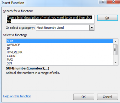
 Many functions and arithmetic operations are pre-programmed in MS Excel. Providing that you know the name and role of a function, you may perform heavy calculations within a few clicks. At any time, click on the symbol
 fx next to the name box to open a dialog box which will help you finding the function that you need (see the picture to the right). If a function is rather common, you may find it immediately in the displayed list or by searching by category. Note that a quick description of the selected function and some info about the syntax and arguments to be used appears in the dialog box. If not, type in a brief description and click Go.
The name/role of the function is often obvious. The function which calculates the average of a series of data is called =AVERAGE(). Less obvious but still logical, the function which calculates the standard deviation of a dataset is called =STDEV(). A bit trickier, the square root of a number will be calculated using the function =SQRT(). Note that functions are always preceded by = and are always followed by parentheses (), even if no argument is necessary. For instance, the function =TODAY() will display the current date in a cell. No argument or data is needed, but the parentheses have to be there, otherwise an error message pops up or the value #NAME? appears in the cell.
Formulas may process a given value (a number directly typed in the formula) or the values placed in other cells in the datasheet. If you just need to display the square root of 121, type =SQRT(121) and press ENTER to obtain the value 11. You may as well display the square root of the result of an arithmetic operation; type =SQRT(100+21) and press ENTER to obatin 11 too. If you need to know the square root of the value contained in E12, type =SQRT(E12).
Many functions may be combined in the same formula. Be careful and check that what you write makes sense, that the syntax is correct and that all parentheses are closed. The longer the formulas, the higher the likelihood of making mistakes. For instance, calculating the standard error of the mean of a range of data may be done in one single, complicated step or in many simple steps. Let’s use an example: fill up the range A1:A10 with random data. Use the cell B1 to calculate the number of values contained in the range (=COUNT(A1:A10)); use B2 to obtain the square root of that count (=SQRT(B1)); calculate the standard deviation of the data in the range A1:A10 in B3 (=STDEV(A1:A10)), and finally find the standard error of the mean in B4 (=B3/B2). Now, in B5, type in the following formula =STDEV(A1:A10)/SQRT(COUNT(A1:A10)). Logically, the value in B4 should be equal to B5… and it is! One line of code was enough to do the job… Watch a video here.
Note that the names of the functions in MS Excel depends of the language in which MS Excel has been installed on the machine. Thus, the function =AVERAGE() becomes =GJENNOMSNITT() on a Norwegian system…
