R

R is a free, powerful statistical and graphical tool which is available for most platforms (Windows, Mac, Linux, FreeBSD, etc.). More than that, it is open source, which means that one can freely modify and adapt R to fit a specific use (providing that one has enough knowledge in terms of programming, of course). In fact, R is not just a software for statistics; it is a language organized around “objects”, linked to data and functions. R is flexible, and it is rather easy to import data for text files (.txt, .csv, …).


hist2
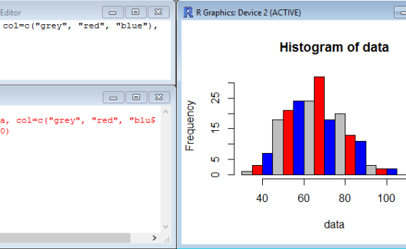
The function hist() is a very simple function which does not require much to build a histogram of frequency (representing the distribution of data series) based on the content of a vector.  Simply typing hist(z), for example, creates a histogram of the vector z made of 10 bars (by default). […]

1. Histogram (of frequency)


pie
You may use pie charts to visualize the proportions of various groups relative to each other and to a whole population. The function that creates pie chart is called pie(x,y) and mainly need two arguments: x which is a numerical vector which contains the size/proportion of the slices, and y […]

2. Pie charts


We have seen in a different section that boxplots are useful charts which represent several features of a dataset: median, quartiles, minimum and maximum, possible outliers… These boxplots become even more useful when they are placed side-by-side in the same chart, and represent different groups to compare. For instance, when […]

3. Multiple Boxplots


Bar graphs (also called bar charts or column charts) are useful to rapidly visualize differences between groups or categories. The relative height of rectangular bars or boxes makes it easy to spot these differences, even when many categories are represented on the same chart. Creating bar graphs does not require […]

4. Bar graphs


Scatter plots display values in the form of dots, squares, crosses, etc corresponding to 2 variables plotted along the X-axis and the Y-axis. In R, all you need is a pair of vectors, one for each variable, and the function plot(). Here is an example where the dataset consists of […]

5. Scatter plots


In R base graphics, there is no function that will directly draw a line chart on its own. Instead, you will need to start with a regular scatter plot with your data represented as dots for example, and then join the dots with lines. While the scatter plot will be […]

6. Line plots


plot
Let’s start easy and create a simple plot of a dataset. The dataset consists of 10 values ranging from 12 to 95 which are stored in the vector y while the vector x contains the series 1:10 that will be used as the X-axis. Here we use the function plot() in […]

2. Starting with a plot


labels
The command plot() may contain several lines of code to tune the display and make the plot more “readable”. For instance, it may be useful to add labels to the Y-axis and X-axis. The arguments to be used are xlab= and ylab= as shown here: [code language=”r”] plot(y~x, xlab="Title for X-axis", […]

3. Adding labels with xlab and ylab


pch col
The default symbol for plotting data elements is an open circle, but you are not obliged to stick to this. The argument pch= (plotting character) allows you to choose the symbol from a list. Check in the list below which symbol you like best and indicate the corresponding number in the […]

5. Modifying symbols


par mar order
When you start playing with the size of the labels and titles, you quickly realize that the frame of the plot becomes too small. It is time to introduce the argument par(mar=c(B,L,T,R)) where B, L, T and R stand for bottom, left, top and right, respectively. Of course you will […]

6. Adjusting margins


coloured titles
Unsurprisingly, the function that adds a title to your plot is called… title(). This function can be “decorated” with several arguments to set the different titles or labels of the chart. Among these are main="text", sub="text", ylab="text", xlab="text", which purposes are to display the main title, a subtitle (secondary title), […]

7. Adding titles and labels


tuning axes
Not only can the text/labels of the axes be tuned, but also the lines, colors, annotations, ticks… The function axis() may be used with various parameters such as col (for the colors), tck (for the length of the ticks), at (for using a vector to indicate the position of the […]

8. Tuning axes


legend
The function legend() is all you need to set up the legend in your chart. It can contain a lot of arguments due to the amount of details such a field may require… The essential arguments are location, title, bg (for background color), cex (for size), text.col (for text color…), legend […]

9. Adding legends


annotations
Two functions are available to add text or notes to your chart: text() and mtext(). Use text() if the text must appear in the graph area, but use mtext() if the text is to be placed in one of the margins. The arguments are location, pos (for the position relative to location), side […]

10. Adding text annotations


abline
Reference lines are useful to visualize a threshold on a chart, or to represent or point at specific values such as mean and median. The function abline( ) draws such a line directly in your chart. abline() needs to know whether the line is horizontal (h=) or vertical (v=) and […]

11. Adding reference lines


clipboard
Once you’ve done your magic, you may be interested in keeping a memory of your masterpiece. This is where the Save as menu becomes useful. Note that the graphic window (the one containing your graph) must be active when saving; if you aren’t sure about it, click once on the […]

13. Saving a graph


combining graphs
A simple function allows you to display multiple charts side-by-side. It can be charts of the same type or of many different sorts; it can be just plots next to each other (lines) or many plots aligned in rows and columns (matrices). That function is called par(mfrow=c(X,Y)) where X is […]

14. Combining graphs


rep()
Here you will find useful functions to create series of numbers to populate your tables and objects. These functions are also quite useful when you want to make a simulation or try functions on a random data set or on a test sample. Note that some functions return integers (numbers […]

1. Creating series


class()
Here are a few functions which are useful to handle and manage objects. ls() lists all the vectors and variables currently stored in memory. [code language=”r”] ls() [/code] Note that the function objects() does exactly the same.   rm() erases from the memory the vector or variable which is named […]

2. Managing objects


dataset[]
head(test) returns by default the first sixth entries in the vector “test”; head(test, 3) returns only the first three entries in the vector “test”. Check the example below: [code language=”r”] test <- c(4,7,9,6,89,45,3,5,78,23,45,0,2,12) test head(test) head(test,  3) [/code]   tail(test) returns the last sixth entries in the vector “test”; tail(test, […]

3. Diverse functions


The function rnorm() generates automatically a series of random values which are normally distributed. This comes quite handy when you want to test functions, statistical analyses or scripts on a random dataset, and you need to be sure that the content is normally distributed beforehand. rnorm() needs the following information: […]

4. Generating random series


NOT a dataframe
A dataframe looks like a two-dimensional matrix. However, unlike a matrix, a dataframe can contain more than numerical values. You can also fill in columns with text values and boolean/logical values (TRUE and FALSE). In a dataframe, the variables, dependent and independent, are placed in columns, while the rows represent the […]

1. Structure and technical properties of a dataframe


attach()
Most of the time you will load the dataframe from an external file, most likely a text file, an excel file or a CSV file (Comma-Separated Values). In that case, you may follow this procedure. In brief, you have to use the command read.xls(), read.table() or read.csv() to open a file and transfer its […]

2. Loading a dataframe


dim dataframe
From here, you can use summary() to get a quick overview of your imported dataframe. summary() offers a reduced, but in fact very informative list of descriptive statistics for each numerical variable, including mean, median, quartiles and minimum/maximum. As for the text and logical variables, a count of each level […]

3. Summary of the dataframe


combination
R gives you the possibility to extract parts of your dataframe. This can be useful to isolate data elements, columns of variables, subsets in your sample… Here are a few commands that create subsets from the dataframe.   extracting single data elements Type the name of the object followed by […]

4. Subscripts of a dataframe


rev()
It is not because you have imported your data from an external source that the order of the observations has to stay as it originally was. You can sort the observations based on ascending or descending values in a column. To do so, you will use the function object.name[order(object.name[,X]),a:b] where X […]

5. Sorting data in the dataframe


When working with big (or huge) dataframes, it might be convenient to create a new dataframe that contains parts of the original one which are selected based on variable names, specific columns or rows, values or ranges… In this post, we will use the following “pseudo-huge” dataframe as an example: […]

6. Working on a subset of the dataframe


It is fairly easy to build a dataframe from scratch in R. All you need is a series of vectors and/or series containing your data and a good recipe! And very often, a good recipe is a simple one… First you have to decide how many columns this dataframe will have, […]

7. Building a dataframe from vectors/series


There are several ways and commands to import data from a file into R. Providing that your data are in an Excel file (.xls, .xlsx), in a text file (.txt), in a comma-separated values file (.csv), you will have to choose the appropriate function. Before going further, check the function […]

2. How to import data into R


With the gsheet R package you can download Google Sheets using a sharing link. You can download the data from the google sheet as a data frame or plain text. Installation [code language=”r”] install.packages(‘gsheet’) [/code] Getting started To download a google sheet, use the following code. The link can be […]

3. How to read data from Google sheets


The name that you choose for your vector may be a single character (such as X) or a word (such as data) but you are allowed/encouraged to be more creative. It may be a more or less abstract sequence of letters and numbers (dataEXT2), a combination of words separated by […]

1. Choosing a name for your vector


matrix coordinates
Objects can also store series of data arranged in the form of a two-dimensional matrix, i.e. an arrangement of data in rows and columns. The function matrix() creates this type of object, but requires a few arguments to properly “draw” the matrix and dispatch the data. First, let’s agree that […]

2. Objects that contain a matrix


long.box array
An array is nothing more than a matrix with more than two dimensions. It is basically a series of two-dimensional matrices “on top of each other”; in other words, a matrix is an array with only two dimensions, or only one layer. To build an array, there is a function […]

3. Objects that contain an array


concatenate
In R, storing data under a specific name is called assignment. There are at least 4 ways to assign data in R: a. with the operator = b. with the operator <- c. with the operator -> d. with the function assign("name,..."). Here is a practical example where single values […]

2. Assigning data elements to a vector


table random list
The table() function in R is used to create… a table. So far, so good. In fact, this is a rather simple function that gathers data and creates a contingency table or frequency table, in other words, a table which counts the number of occurrences of any unique value in […]

5. Objects that contain a table


Dataframes are a central type of object when working with statistics in R. They are actually simple two-dimensional matrices arrays which contain your data, arranged in a rather specific manner. They are in a way so special when working with statistics in R that they deserve their own, dedicated page. […]

6. Objects that contain a dataframe


multiply vectors size
Now that you have stored values or data elements in vectors, you may start working with/on these vectors. The simplest operations that you can perform are regular arithmetical operations such as addition, subtraction, multiplication and division. Here is an example where the vector data1 is multiplied by 5: [code language=”r”] […]

3. Simple arithmetical operations involving vectors


script to console2
When starting up R, you might be confronted with a feeling of “being lost at sea”. Few icons, few menus, not much of a welcoming screen… just a menu bar and the R console. You’ll soon realize that you can write “stuff” in this R console. You can write arithmetical operations, […]

1. Start working with the editor, not the console


combination
It is fairly easy to perform simple arithmetic operations in R. You simply need to type in the operations as command directly in the editor (script), right after the > sign, and press ENTER to validate. Use +, -, * and / for additions, subtractions, multiplications and divisions, respectively. Try to […]

2. Using R as a calculator


if nothing happens
Sooner or later, everyone needs help… and working with R does not constitute any exception. There are several ways to get help with R. In R: As indicated in the R console when starting up R, you may get help by typing help(). This command opens immediately a new page/tab in […]

3. Finding help in R


setwd()
When working with multiple datasets belonging to different projects, it is best to keep things organised. By this, you have to understand that it is best to save your data files, processed datasets and the content of the workspace in R (script, etc) in a specific folder, the working directory. […]

4. Setting up a working directory


library()
Because it is open source, R has a constantly growing list of updated packages to be added to the core functions of the program. The packages are usually built by advanced users and programmers who wish to add functionalities, to simplify procedures that may require a long list of commands… […]

5. Installing packages


concatenate vectors
Not only you can perform arithmetic operations to vectors, but you can also “merge” them or combine them. To do so, simply use the concatenate function c(...) to concatenate the two vectors,: [code language=”r”] data1 = c("aa","bb","cc","dd","ee") data2 = c(10,20) c(data1,data2) [/code]   The example above is a bit particular […]

4. Combining vectors


citation
If your research project, data and results are to be published and you have used R to perform calculations, you will have to cite R in the appropriate manner. There is a function in R which provides you with the proper citation. Just type citation() to obtain the following screen: [code language=”r”] […]

6. Citing R in publications